Contents
2. References
2.1. Tools related to network (e.g., protein networks)
Utilities related to networks (e.g., protein)
-
class
Complexes(organism='Homo sapiens', verbose=True, cache=False)[source]¶ Manipulate complexes of Proteins
This class uses Intact Complex database to extract information about complexes of proteins.
When creating an instance, the default organism is “Homo sapiens”. The organism can be set to another one during the instanciation or later:
>>> from biokit.network.complexes import Complexes
>>> c = Complexes(organism='Homo sapiens')
>>> c.organism = 'Rattus norvegicus'
Valid organisms can be found in
organisms. When changing the organism, a request to the Intact database is sent, which may take some time to update. Once done, information related to this organism is stored in thedfattribute, which is a Pandas dataframe. It contains 4 columns. Here is for example one row:complexAC EBI-2660609 complexName COP9 signalosome variant 1 description Essential regulator of the ubiquitin (Ubl) con... organismName Homo sapiens; 9606
This is basic information but once a complex accession (e.g., EBI-2660609) is known, you can retrieve detailled information. This is done automatically for all the accession when needed. The first time, it will take a while (20 seconds for 250 accession) but will be cache for this instance.
The
complexescontains all details about the entries found indf. It is a dictionary where keys are the complex accession. For instance:>>> c.complexes['EBI-2660609']
In general, one is interested in the participants of the complex, that is the proteins that form the complex. Another attribute is set for you:
>>> c.participants['EBI-2660609']
Finally, you may even want to obtain just the identifier of the participants for each complex. This is stored in the
identifiers:>>> c.identifiers['EBI-2660609']
Note however, that the identifiers are not neceseraly uniprot identifiers. Could be ChEBI or sometimes even set to None. The
strict_filter()removes the complexes with less than 2 (strictly) uniprot identifiers.Some basic statistics can be printed with
stats()that indeticates the number of complexes, number of identifiers in those complexes ,and number of unique identifiers. A histogram of number of appearance of each identifier is also shown.The
hist_participants()shows the number of participants per complex.Finally, the meth:search_complexes can be used in the context of logic modelling to infer the AND gates from a list of uniprot identifiers provided by the user. See
search_complexes()for details.Access to the Intact Complex database is performed using the package BioServices provided in Pypi.
Constructor
Parameters: -
complexes¶ Getter of the complexes (full details
-
hist_participants()[source]¶ Histogram of the number of participants per complexes
Returns: a dictionary with complex identifiers as keys and number of participants as values from biokit.network.complexes import Complexes c = Complexes() c.hist_participants()
-
identifiers¶ Getter of the identifiers of the complex participants
-
organism¶ Getter/Setter of the organism
-
organisms= None¶ list of valid organisms found in the database
-
participants¶ Getter of the complex participants (full details)
-
remove_homodimers()[source]¶ Remove identifiers that are None or starts with CHEBI and keep complexes that have at least 2 participants
Returns: list of complex identifiers that have been removed.
-
search(name)[source]¶ Search for a unique identifier (e.g. uniprot) in all complexes
Returns: list of complex identifiers where the name was found
-
search_complexes(user_species, verbose=False)[source]¶ - Given a list of uniprot identifiers, return complexes and
- possible complexes.
Parameters: user_species (list) – list of uniprot identifiers to be found in the complexes Returns: two dictionaries. First one contains the complexes for which all participants have been found in the user_species list. The second one contains complexes for which some participants (not all) have been found in the user_species list.
-
stats()[source]¶ Prints some stats about the number of complexes and histogram of the number of appearances of each species
-
valid_organisms= None¶ list of valid organisms found in the database
-
2.2. Common visualisation tools
Plotting tools
biokit.viz.corrplot.Corrplot(data[, na]) |
An implementation of correlation plotting tools (corrplot) |
biokit.viz.hinton.hinton(df[, fig, shrink, …]) |
Hinton plot (simplified version of correlation plot) |
biokit.viz.hist2d.Hist2D(x[, y, verbose]) |
2D histogram |
biokit.viz.imshow.Imshow(x[, verbose]) |
Wrapper around the matplotlib.imshow function |
biokit.viz.scatter.ScatterHist(x[, y, verbose]) |
Scatter plots and histograms |
biokit.viz.volcano.Volcano([fold_changes, …]) |
Volcano plot |
biokit.viz.heatmap.Heatmap([data, …]) |
Heatmap and dendograms of an input matrix |
Corrplot utilities
| author: | Thomas Cokelaer |
|---|---|
| references: | http://cran.r-project.org/web/packages/corrplot/vignettes/corrplot-intro.html |
-
class
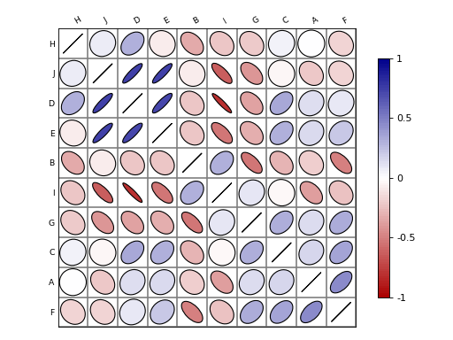
Corrplot(data, na=0)[source]¶ An implementation of correlation plotting tools (corrplot)
Here is a simple example with a correlation matrix as an input (stored in a pandas dataframe):
# create a correlation-like data set stored in a Pandas' dataframe.
import string
# letters = string.uppercase[0:10] # python2
letters = string.ascii_uppercase[0:10]
import pandas as pd
df = pd.DataFrame(dict(( (k, np.random.random(10)+ord(k)-65) for k in letters)))

# and use corrplot
from biokit.viz import corrplot
c = corrplot.Corrplot(df)
c.plot()
(Source code, png, hires.png, pdf)
See also
All functionalities are covered in this notebook
Constructor
Plots the content of square matrix that contains correlation values.
Parameters: - data – input can be a dataframe (Pandas), or list of lists (python) or
a numpy matrix. Note, however, that values must be between -1 and 1. If not,
or if the matrix (or list of lists) is not squared, then correlation is
computed. The data or computed correlation is stored in
dfattribute. - compute_correlation (bool) – if the matrix is non-squared or values are not bounded in -1,+1, correlation is computed. If you do not want that behaviour, set this parameter to False. (True by default).
- na – replace NA values with this value (default 0)
The
paramscontains some tunable parameters for the colorbar in theplot()method.# can be a list of lists, the correlation matrix is then a 2x2 matrix c = corrplot.Corrplot([[1,1], [2,4], [3,3], [4,4]])
-
df= None¶ The input data is stored in a dataframe and must therefore be compatible (list of lists, dictionary, matrices…)
-
order(method='complete', metric='euclidean', inplace=False)[source]¶ Rearrange the order of rows and columns after clustering
Parameters: - method – any scipy method (e.g., single, average, centroid, median, ward). See scipy.cluster.hierarchy.linkage
- metric – any scipy distance (euclidean, hamming, jaccard) See scipy.spatial.distance or scipy.cluster.hieararchy
- inplace (bool) – if set to True, the dataframe is replaced
You probably do not need to use that method. Use
plot()and the two parameters order_metric and order_method instead.
-
plot(fig=None, grid=True, rotation=30, lower=None, upper=None, shrink=0.9, facecolor='white', colorbar=True, label_color='black', fontsize='small', edgecolor='black', method='ellipse', order_method='complete', order_metric='euclidean', cmap=None, ax=None, binarise_color=False)[source]¶ plot the correlation matrix from the content of
df(dataframe)By default, the correlation is shown on the upper and lower triangle and is symmetric wrt to the diagonal. The symbols are ellipses. The symbols can be changed to e.g. rectangle. The symbols are shown on upper and lower sides but you could choose a symbol for the upper side and another for the lower side using the lower and upper parameters.
Parameters: - fig – Create a new figure by default. If an instance of an existing figure is provided, the corrplot is overlayed on the figure provided. Can also be the number of the figure.
- grid – add grid (Defaults to grey color). You can set it to False or a color.
- rotation – rotate labels on y-axis
- lower – if set to a valid method, plots the data on the lower left triangle
- upper – if set to a valid method, plots the data on the upper left triangle
- shrink (float) – maximum space used (in percent) by a symbol. If negative values are provided, the absolute value is taken. If greater than 1, the symbols wiill overlap.
- facecolor – color of the background (defaults to white).
- colorbar – add the colorbar (defaults to True).
- label_color (str) – (defaults to black).
- fontsize – size of the fonts defaults to ‘small’.
- method – shape to be used in ‘ellipse’, ‘square’, ‘rectangle’, ‘color’, ‘text’, ‘circle’, ‘number’, ‘pie’.
- order_method – see
order(). - order_metric – see : meth:order.
- cmap – a valid cmap from matplotlib or colormap package (e.g., ‘jet’, or ‘copper’). Default is red/white/blue colors.
- ax – a matplotlib axes.
The colorbar can be tuned with the parameters stored in
params.Here is an example. See notebook for other examples:
c = corrplot.Corrplot(dataframe)
c.plot(cmap=('Orange', 'white', 'green'))
c.plot(method='circle')
c.plot(colorbar=False, shrink=.8, upper='circle'  )
- data – input can be a dataframe (Pandas), or list of lists (python) or
a numpy matrix. Note, however, that values must be between -1 and 1. If not,
or if the matrix (or list of lists) is not squared, then correlation is
computed. The data or computed correlation is stored in
Scatter plots
| author: | Thomas Cokelaer |
|---|
-
class
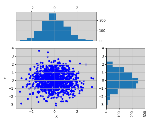
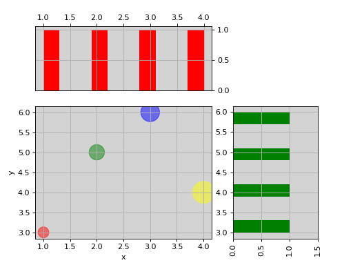
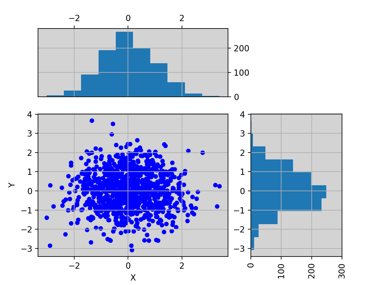
ScatterHist(x, y=None, verbose=True)[source]¶ Scatter plots and histograms
constructor
Parameters: - x – if x is provided, it should be a dataframe with 2 columns. The first one will be used as your X data, and the second one as the Y data
- y –
- verbose –
-
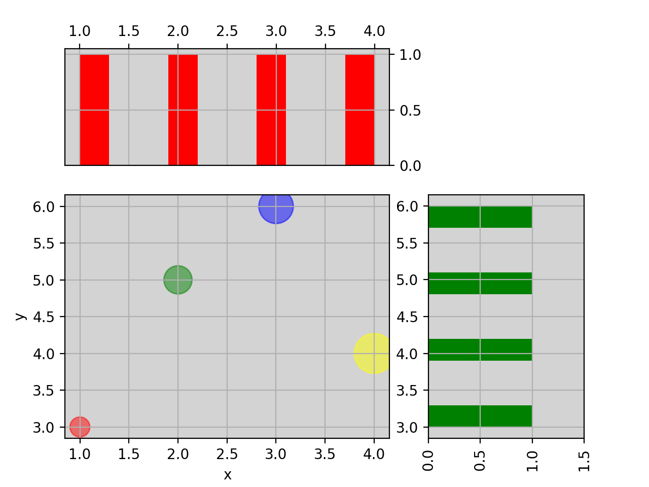
plot(kargs_scatter={'c': 'b', 's': 20}, kargs_grids={}, kargs_histx={}, kargs_histy={}, scatter_position='bottom left', width=0.5, height=0.5, offset_x=0.1, offset_y=0.1, gap=0.06, facecolor='lightgrey', grid=True, show_labels=True, **kargs)[source]¶ Scatter plot of set of 2 vectors and their histograms.
Parameters: - x – a dataframe or a numpy matrix (2 vectors) or a list of 2 items, which can be a mix of list or numpy array. if size and/or color are found in the columns dataframe, those columns will be used in the scatter plot. kargs_scatter keys c and s will then be ignored. If a list of lists, x will be the first row and y the second row.
- y – if x is a list or an array, then y must also be provided as a list or an array
- kargs_scatter – a dictionary with pairs of key/value accepted by matplotlib.scatter function. Examples is a list of colors or a list of sizes as shown in the examples below.
- kargs_grid – a dictionary with pairs of key/value accepted by the maplotlib.grid (applied on histogram and axis at the same time)
- kargs_histx – a dictionary with pairs of key/value accepted by the matplotlib.histogram
- kargs_histy – a dictionary with pairs of key/value accepted by the matplotlib.histogram
- kargs – other optional parameters are hold, facecolor.
- scatter_position – can be ‘bottom right/bottom left/top left/top right’
- width – width of the scatter plot (value between 0 and 1)
- height – height of the scatter plot (value between 0 and 1)
- offset_x –
- offset_y –
- gap – gap between the scatter and histogram plots.
- grid – defaults to True
Returns: the scatter, histogram1 and histogram2 axes.
import pylab
import pandas as pd
X = pylab.randn(1000)
Y = pylab.randn(1000)
df = pd.DataFrame({'X':X, 'Y':Y})

from biokit.viz import ScatterHist
ScatterHist(df).plot()
(Source code, png, hires.png, pdf)
from biokit.viz import ScatterHist
ScatterHist(x=[1,2,3,4], y=[3,5,6,4]).plot(
    kargs_scatter={
        's':[200,400,600,800],
        'c': ['red', 'green', 'blue', 'yellow'],
        'alpha':0.5},
    kargs_histx={'color': 'red'},
    kargs_histy={'color': 'green'})
(Source code, png, hires.png, pdf)
See also
Imshow utility
-
imshow(x, interpolation='None', aspect='auto', cmap='hot', tight_layout=True, colorbar=True, fontsize_x=None, fontsize_y=None, rotation_x=90, xticks_on=True, yticks_on=True, **kargs)[source]¶ Alias to the class
Imshow
-
class
Imshow(x, verbose=True)[source]¶ Wrapper around the matplotlib.imshow function
Very similar to matplotlib but set interpolation to None, and aspect to automatic and accepts input as a dataframe, in whic case x and y labels are set automatically.
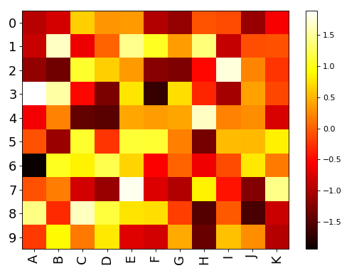
import pandas as pd
data = dict([ (letter,np.random.randn(10)) for letter in 'ABCDEFGHIJK'])
df = pd.DataFrame(data)

from biokit import Imshow
im = Imshow(df)
im.plot()
(Source code, png, hires.png, pdf)

constructor
Parameters: x – input dataframe (or numpy matrix/array). Must be squared. -
plot(interpolation='None', aspect='auto', cmap='hot', tight_layout=True, colorbar=True, fontsize_x=None, fontsize_y=None, rotation_x=90, xticks_on=True, yticks_on=True, **kargs)[source]¶ wrapper around imshow to plot a dataframe
Parameters: - interpolation – set to None
- aspect – set to ‘auto’
- cmap – colormap to be used.
- tight_layout –
- colorbar – add a colobar (default to True)
- fontsize_x – fontsize on xlabels
- fontsize_y – fontsize on ylabels
- rotation_x – rotate labels on xaxis
- xticks_on – switch off the xticks and labels
- yticks_on – switch off the yticks and labels
-
Heatmap and dendograms
-
class
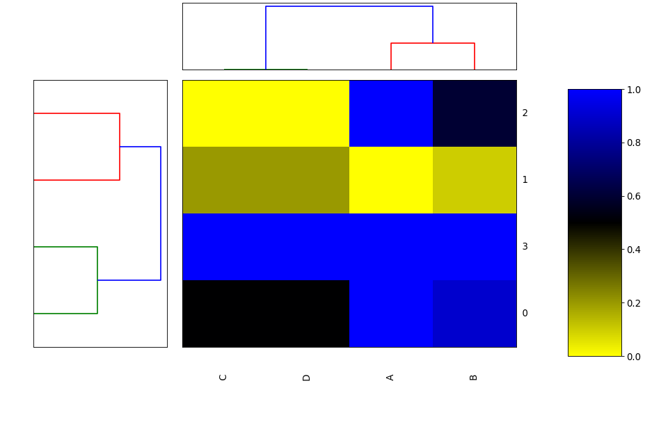
Heatmap(data=None, row_method='complete', column_method='complete', row_metric='euclidean', column_metric='euclidean', cmap='yellow_black_blue', col_side_colors=None, row_side_colors=None, verbose=True)[source]¶ Heatmap and dendograms of an input matrix
A heat map is an image representation of a matrix with a dendrogram added to the left side and to the top. Typically, reordering of the rows and columns according to some set of values (row or column means) within the restrictions imposed by the dendrogram is carried out.
from biokit.viz import heatmap
df = heatmap.get_heatmap_df()
h = heatmap.Heatmap(df)
h.plot()
(Source code, png, hires.png, pdf)
Warning
in progress
constructor
Parameters: data – a dataframe or possibly a numpy matrix. Todo
if row_method id none, no ordering in the dendogram
-
column_method
-
column_metric
-
df
-
frame
-
plot(num=1, cmap=None, colorbar=True, vmin=None, vmax=None, colorbar_position='right', gradient_span='None')[source]¶ Parameters: gradient_span – None is default in R Using:
df = pd.DataFrame({'A':[1,0,1,1],
                   'B':[.9,0.1,.6,1],
                'C':[.5,.2,0,1],
                'D':[.5,.2,0,1]})
and
h = Heatmap(df)
h.plot(vmin=0, vmax=1.1)
we seem to get the same as in R wiht
df = data.frame(A=c(1,0,1,1), B=c(.9,.1,.6,1), C=c(.5,.2,0,1), D=c(.5,.2,0,1))
heatmap((as.matrix(df)), scale='none')
Todo
right now, the order of cols and rows is random somehow. could be ordered like in heatmap (r) byt mean of the row and col or with a set of vector for col and rows.
heatmap((as.matrix(df)), Rowv=c(3,2), Colv=c(1), scale=’none’)
gives same as:
df = get_heatmap_df()
h = heatmap.Heatmap(df)
h.plot(vmin=-0, vmax=1.1)
-
row_method
-
row_metric
-
Hinton plot
| author: | Thomas Cokelaer |
|---|
-
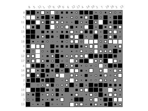
hinton(df, fig=1, shrink=2, method='square', bgcolor='grey', cmap='gray_r', binarise_color=True)[source]¶ Hinton plot (simplified version of correlation plot)
Parameters: - df – the input data as a dataframe or list of items (list, array). See
Corrplotfor details. - fig – in which figure to plot the data
- shrink – factor to increase/decrease sizes of the symbols
- method – set the type of symbols for each coordinates. (default to square). See
Corrplotfor more details. - bgcolor – set the background and label colors as grey
- cmap – gray color map used by default
- binarise_color – use only two colors. One for positive values and one for negative values.
from biokit.viz import hinton
df = np.random.rand(20, 20) - 0.5
hinton(df)
(Source code, png, hires.png, pdf)

Note
Idea taken from a matplotlib recipes http://matplotlib.org/examples/specialty_plots/hinton_demo.html but solely using the implementation within
CorrplotSee also
Note
Values must be between -1 and 1. No sanity check performed.
- df – the input data as a dataframe or list of items (list, array). See
Volcano plot
-
class
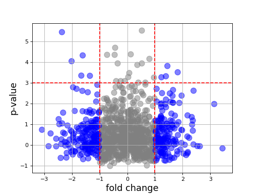
Volcano(fold_changes=None, pvalues=None, color=None)[source]¶ Volcano plot
In essence, just a scatter plot with annotations.
import numpy as np
fc = np.random.randn(1000)
pvalue = np.random.randn(1000)

from biokit import Volcano
v = Volcano(fc, -np.log10(pvalue**2))
v.plot(pvalue_threshold=3)
(Source code, png, hires.png, pdf)
constructor
Parameters: -
plot(size=100, alpha=0.5, marker='o', fontsize=16, xlabel='fold change', ylabel='p-value', pvalue_threshold=1.5, fold_change_threshold=1)[source]¶ Parameters: - size – size of the markers
- alpha – transparency of the marker
- fontsize –
- xlabel –
- ylabel –
- pvalue_threshold – adds an horizontal dashed line at the threshold provided.
- fold_change_threshold – colors in grey the absolute fold changes below a given threshold.
-
2D histograms
-
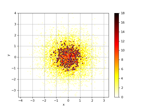
class
Hist2D(x, y=None, verbose=False)[source]¶ 2D histogram
from numpy import random
from biokit.viz import hist2d
X = random.randn(10000)
Y = random.randn(10000)
h = hist2d.Hist2D(X,Y)
h.plot(bins=100, contour=True)
(Source code, png, hires.png, pdf)

constructor
Parameters: - x – an array for X values. See
VizInput2Dfor details. - y – an array for Y values. See
VizInput2Dfor details.
-
plot(bins=100, cmap='hot_r', fontsize=10, Nlevels=4, xlabel=None, ylabel=None, norm=None, range=None, normed=False, colorbar=True, contour=True, grid=True, **kargs)[source]¶ plots histogram of mean across replicates versus coefficient variation
Parameters: - bins (int) – binning for the 2D histogram (either a float or list of 2 binning values).
- cmap – a valid colormap (defaults to hot_r)
- fontsize – fontsize for the labels
- Nlevels (int) – must be more than 2
- xlabel (str) – set the xlabel (overwrites content of the dataframe)
- ylabel (str) – set the ylabel (overwrites content of the dataframe)
- norm – set to ‘log’ to show the log10 of the values.
- normed – normalise the data
- range – as in pylab.Hist2D : a 2x2 shape [[-3,3],[-4,4]]
- contour – show some contours (default to True)
- grid (bool) – Show unerlying grid (defaults to True)
If the input is a dataframe, the xlabel and ylabel will be populated with the column names of the dataframe.
- x – an array for X values. See
Core function for the plotting tools
2.3. Tools to handle R packages
utilities related to R language (e.g., RPackageManager, RSession)
-
class
RSession(RExecutable='R', max_len=1000, use_dict=None, host='localhost', user=None, ssh='ssh', verbose=False, return_err=True)[source]¶ Interface to a R session
This class uses the pyper package to provide an access to R (via a subprocess). You can call R script and get back the results into the session as Python objects. Returned objects may be transformed into numpy arrays or Pandas datafranes.
Here is a very simple example but any complex R scripts can be provided inside the
run()method:from biokit.rtools import RSession session = RSession() session.run("mylist = c(1,2,3)") a = session("mylist") # access to the R object a.sum() # a is numpy array
There are different ways to access to the R object:
# getter
session['a']
# method-wise:
session.get('a')
# attribute:
session.a
For now, this is just to inherit from pyper.R class but there is no additional features. This is to create a common API.
Parameters: - RCMD (str) – the name of the R executable
- max_len – define the upper limitation for the length of command string. A command string will be passed to R by a temporary file if it is longer than this value.
- host – The computer name (or IP) on which the R interpreter is installed. The value “localhost” means that the R locates on the the localhost computer. On POSIX systems (including Cygwin environment on Windows), it is possible to use R on a remote computer if the command “ssh” works. To do that, the user need set this value, and perhaps the parameter “user”.
- user – The user name on the remote computer. This value need to be set only if the user name is different on the remote computer. In interactive environment, the password can be input by the user if prompted. If running in a program, the user need to be able to login without typing password! (i.e., you need to set your SSH keys)
- ssh – The program to login to remote computer.
- kargs – must be empty. Error raised otherwise
-
biocLite(package=None, suppressUpdates=True, verbose=True)[source]¶ Install a bioconductor package
This function does not work like the R function. Only a few options are implemented so far. However, you can use rcode function directly if needed.
Parameters: Returns: True if update is required or the required package is installed and could be imported. False otherwise.
>>> from biokit.viz.rtools import biocLite
>>> biocLite("CellNOptR")
-
class
RPackage(name, version_required=None, install=False, verbose=False)[source]¶ >>> from biokit.rtools import package >>> p = package.RPackage('CellNOptR') >>> p.isinstalled True >>> p.version '1.11.3'
Todo
do we need the version_required attribute/parameter anywhere ?
Note
R version includes dashes, which are not recognised by distutils so they should be replaced.
-
isinstalled
-
version
-
-
install_package(query, dependencies=False, verbose=True, repos='http://cran.univ-paris1.fr/')[source]¶ Install a R package
Parameters: - query (str) – It can be a valid URL to a R package (tar ball), a CRAN package, a path to a R package (tar ball), or simply the directory containing a R package source.
- dependencies (bool) –
- repos – if provided, install_packages automatically select the provided repositories otherwise a popup window will ask you to select a repo
>>> rtools.install_package("path_to_a_valid_Rpackage.tar.gz")
>>> rtools.install_package("http://URL_to_a_valid_Rpackage.tar.gz")
>>> rtools.install_package("hash") # a CRAN package
>>> rtools.install_package("path to a valid R package directory")
See also
biokit.rtools.RPackageManager
-
class
RPackageManager(verbose=True)[source]¶ Implements a R package manager from Python
So far you can install a package (from source, or CRAN, or biocLite)
pm = PackageManager()
[(x, pm.installed[x][2]) for x in pm.installed.keys()]
You can access to all information within a dataframe called packages where indices are the name packages. Some aliases are provided as attributes (e.g., available, installed)
-
available
-
biocLite(package=None, suppressUpdates=True, verbose=False)[source]¶ Installs one or more biocLite packages
Parameters: package – a package name (string) or list of package names (list of strings) that will be installed from BioConductor. If package is set to None, all packages already installed will be updated.
-
cran_repos= 'http://cran.univ-lyon1.fr/'
-
install(pkg, require=None, update=True, reinstall=False)[source]¶ install a package automatically scanning CRAN and biocLite repos
if require is not set and update is True, when a newest version of a package is available, it is installed
-
installed
-
packages
-
Code use by pyper module original version available from pyper pacakge on pip
2.4. Genomics
Sequence related (Generic, DNA, RNA)
-
class
Sequence(data='')[source]¶ Common data structure to all sequences (e.g.,
DNA())A sequence is a string contained in the
_data. If you manipulate this attribute, you should also changed the_N(length of the string) and set_counterto None.Sequences can be concatenated easily. You can also add a string or numpy array or pandas time series to an existing sequence:
d1 = Sequence('ACGT')
d2 = Sequence('ACGT')
Note that there is a
check()method, which is not called during the instanciation but is called when adding sequences together. Each type of sequence (e.g., Sequence, DNA, RNA) has its own symbols. So you cannot add a DNA sequence with a RNA sequence for instance. Those are valid operation:>>> d1 = Sequence('ACGT') >>> d1 += 'AAAA' >>> d1 + d1 >>> "AAAA" + d1
-
N
-
counter¶ return counter of the letters
-
hamming_distance(other)[source]¶ Return hamming distance between this sequence and another sequence
The Hamming distance between s and t, denoted dH(s,t), is the number of corresponding symbols that differ in s and t.
>>> d1 = 'GAGCCTACTAACGGGAT'
>>> d2 = 'CATCGTAATGACGGCCT'
>>> s = Sequence(d1)
>>> s.hamming_distance(d2)
7
-
sequence¶ returns a copy of the sequence
-
DNA sequence
-
class
DNA(data='')[source]¶ a DNA
Sequence.You can add DNA sequences together:
>>> from biokit import DNA
>>> s1 = DNA('ACGT')
>>> s2 = DNA('AAAA')
>>> s1 + s2
Sequence: ACGTAAAA (length 8)
-
complement
-
gc_content(letters='CGS')[source]¶ Returns the G+C content in percentage.
Copes mixed case sequences, and with the ambiguous nucleotide S (G or C) when counting the G and C content.
>>> from biokit.sequence.dna import DNA
>>> d = DNA("ACGTSAAA")
>>> d.gc_content()
0.375
-
reverse_complement
-
RNA sequence
-
class
RNA(sequence='')[source]¶ -
complement
-
gc_content(letters='CGS')[source]¶ Returns the G+C content in percentage.
Copes mixed case sequences, and with the ambiguous nucleotide S (G or C) when counting the G and C content.
>>> from biokit.sequence.dna import RNA
>>> d = RNA("ACGTSAAA")
>>> d.gc_content()
0.375
-
reverse_complement
-
-
class
Peptide(data)[source]¶ a Peptide
Sequence.You can add Peptide sequences together:
>>> from biokit import DNA
>>> s1 = Peptide('ACGT')
>>> s2 = Peptide('AAAA')
>>> s1 + s2
Sequence: ACGTAAAA (length 8)
Note
redundant with Sequence but may evolve in the future.
-
class
Taxon(taxid)[source]¶ Some codecs
-
to_genbank(retmax=10000)[source]¶ Draft: from a TaxID, uses EUtils to retrieve the GenBank identifiers
Inspiration: https://gist.github.com/fjossinet/5673672
-
-
class
Taxonomy(verbose=True, online=True)[source]¶ This class should ease the retrieval and manipulation of Taxons
There are many resources to retrieve information about a Taxon. For instance, from BioServices, one can use UniProt, Ensembl, or EUtils. This is convenient to retrieve a Taxon (see
fetch_by_name()andfetch_by_id()that rely on Ensembl). However, you can also download a flat file from EBI ftp server, which stores a set or records (1.3M at the time of the implementation).Note that the Ensembl database does not seem to be as up to date as the flat files but entries contain more information.
for instance taxon 2 is in the flat file but not available through the
fetch_by_id(), which uses ensembl.So, you may access to a taxon in 2 different ways getting differnt dictionary. However, 3 keys are common (id, parent, scientific_name)
>>> t = taxonomy.Taxonomy()
>>> t.fetch_by_id(9606)   # Get a dictionary from Ensembl
>>> t.records[9606] # or just try with the get
>>> t[9606]
>>> t.get_lineage(9606)
constructor
Parameters: offline – if you do not have internet, the connction to Ensembl may hang for a while and fail. If so, set offline to True -
fetch_by_id(taxon)[source]¶ Search for a taxon by identifier
:return; a dictionary.
>>> ret = s.search_by_id('10090')
>>> ret['name']
'Mus Musculus'
-
fetch_by_name(name)[source]¶ Search a taxon by its name.
Parameters: name (str) – name of an organism. SQL cards possible e.g., _ and % characters. Returns: a list of possible matches. Each item being a dictionary. >>> ret = s.search_by_name('Mus Musculus') >>> ret[0]['id'] 10090
-
get_lineage(taxon)[source]¶ Get lineage of a taxon
Parameters: taxon (int) – a known taxon Returns: list containing the lineage
-
2.5. Stats
Generic statistical tools
-
class
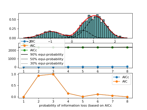
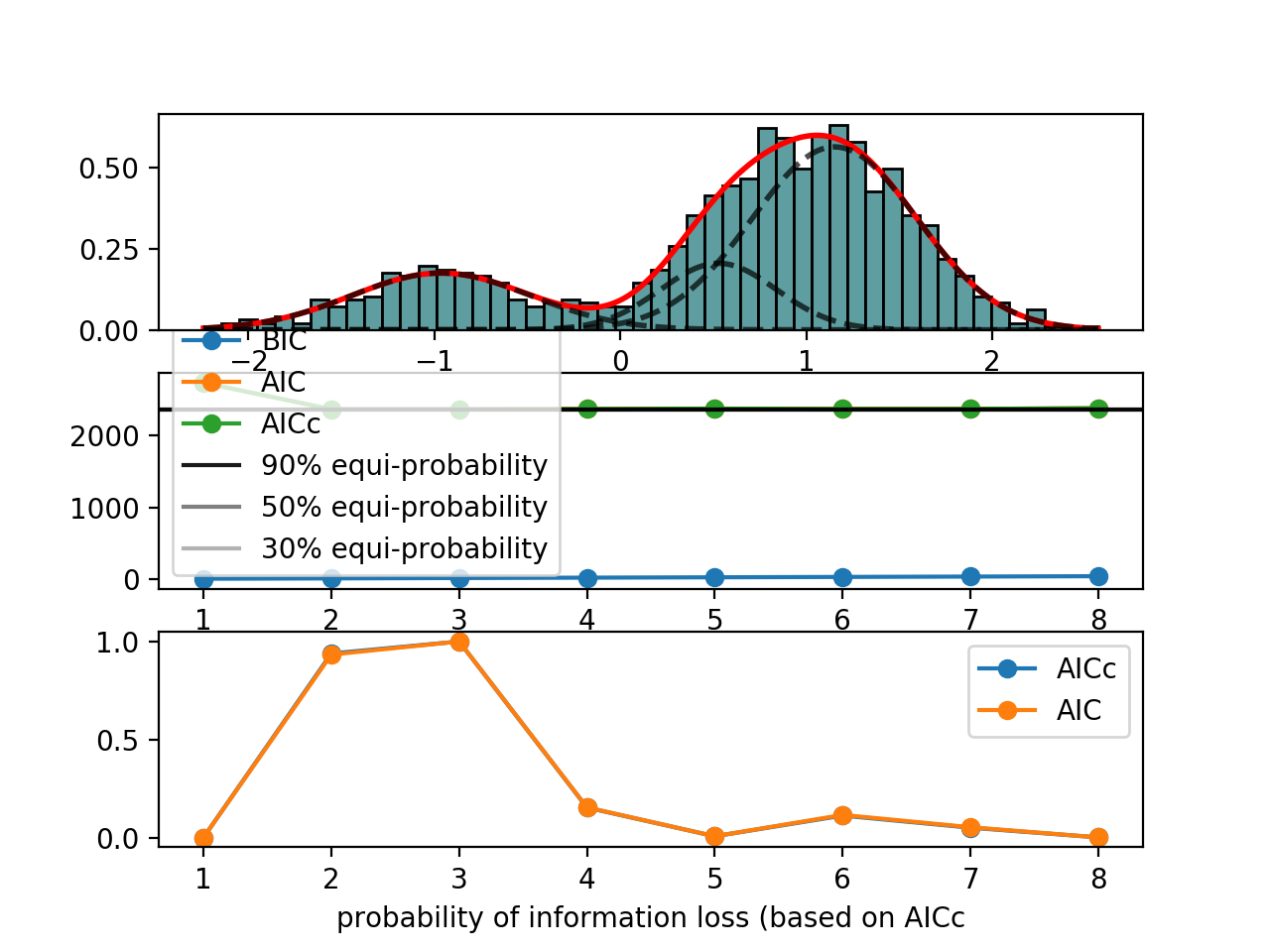
AdaptativeMixtureFitting(data, method='Nelder-Mead')[source]¶ Automatic Adaptative Mixture Fitting
from biokit.stats.mixture import AdaptativeMixtureFitting, GaussianMixture
m = GaussianMixture(mu=[-1,1], sigma=[0.5,0.5], mixture=[0.2,0.8])
amf = AdaptativeMixtureFitting(m.data)
amf.run(kmin=1, kmax=6)
amf.diagnostic(k=amf.best_k)
(Source code, png, hires.png, pdf)
-
class
EM(data, model=None, max_iter=100)[source]¶ Expectation minimization class to estimate parameters of GMM
from biokit.stats.mixture import GaussianMixture, EM
m = GaussianMixture(mu=[-1,1], sigma=[0.5,0.5], mixture=[0.2,0.8])
em = EM(m.data)
em.estimate(k=2)
em.plot()
(Source code, png, hires.png, pdf)
constructor
Parameters: - data –
- model – not used. Model is the
GaussianMixtureModelbut could be other model. - max_iter (int) – max iteration for the minization
-
class
Fitting(data, k=2, method='Nelder-Mead')[source]¶ Base class for
EMandGaussianMixtureFittingconstructor
Parameters: -
k
-
model
-
-
class
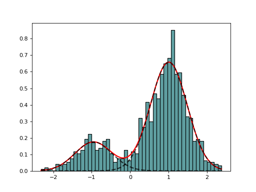
GaussianMixture(mu=[-1, 1], sigma=[1, 1], mixture=[0.5, 0.5], N=1000)[source]¶ Creates a mix of Gaussian distribution
from biokit.stats.mixture import GaussianMixture
m = GaussianMixture(mu=[-1,1], sigma=[0.5, 0.5], mixture=[.2, .8], N=1000)
m.plot()
(Source code, png, hires.png, pdf)

constructor
Parameters:
-
class
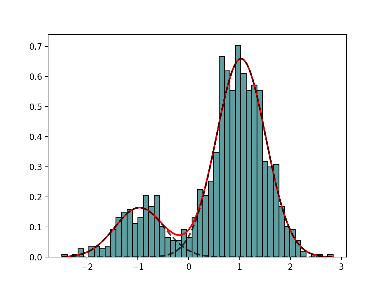
GaussianMixtureFitting(data, k=2, method='Nelder-Mead')[source]¶ GaussianMixtureFitting using scipy minization
from biokit.stats.mixture import GaussianMixture, GaussianMixtureFitting
m = GaussianMixture(mu=[-1,1], sigma=[0.5,0.5], mixture=[0.2,0.8])
mf = GaussianMixtureFitting(m.data)
mf.estimate(k=2)
mf.plot()
(Source code, png, hires.png, pdf)

Here we use the function minimize() from scipy.optimization. The list of (currently) available minimization methods is ‘Nelder-Mead’ (simplex), ‘Powell’, ‘CG’, ‘BFGS’, ‘Newton-CG’,> ‘Anneal’, ‘L-BFGS-B’ (like BFGS but bounded), ‘TNC’, ‘COBYLA’, ‘SLSQPG’.
-
estimate(guess=None, k=None, maxfev=20000.0, maxiter=1000.0, bounds=None)[source]¶ guess is a list of parameters as expected by the model
guess = {‘mus’:[1,2], ‘sigmas’: [0.5, 0.5], ‘pis’: [0.3, 0.7] }
-
method
-
Akaike and other criteria
-
AIC(L, k, logL=False)[source]¶ Return Akaike information criterion (AIC)
Parameters: Suppose that we have a statistical model of some data, from which we computed its likelihood function and let
 be the number of parameters in the model
(i.e. degrees of freedom). Then the AIC value is:
be the number of parameters in the model
(i.e. degrees of freedom). Then the AIC value is:
Given a set of candidate models for the data, the preferred model is the one with the minimum AIC value. Hence AIC rewards goodness of fit (as assessed by the likelihood function), but it also includes a penalty that is an increasing function of the number of estimated parameters. The penalty discourages overfitting.
Suppose that there are R candidate models AIC1, AIC2, AIC3, AICR. Let AICmin be the minimum of those values. Then, exp((AICmin - AICi)/2) can be interpreted as the relative probability that the ith model minimizes the (estimated) information loss.
Suppose that there are three candidate models, whose AIC values are 100, 102, and 110. Then the second model is exp((100 - 102)/2) = 0.368 times as probable as the first model to minimize the information loss. Similarly, the third model is exp((100 - 110)/2) = 0.007 times as probable as the first model, which can therefore be discarded.
With the remaining two models, we can (1) gather more data, (2) conclude that the data is insufficient to support selecting one model from among the first two (3) take a weighted average of the first two models, with weights 1 and 0.368.
The quantity exp((AIC_{min} - AIC_i)/2) is the relative likelihood of model i.
If all the models in the candidate set have the same number of parameters, then using AIC might at first appear to be very similar to using the likelihood-ratio test. There are, however, important distinctions. In particular, the likelihood-ratio test is valid only for nested models, whereas AIC (and AICc) has no such restriction.
Reference: Burnham, K. P.; Anderson, D. R. (2002), Model Selection and Multimodel Inference: A Practical Information-Theoretic Approach (2nd ed.), Springer-Verlag, ISBN 0-387-95364-7.
-
AICc(L, k, n, logL=False)[source]¶ AICc criteria
Parameters: AIC with a correction for finite sample sizes. The formula for AICc depends upon the statistical model. Assuming that the model is univariate, linear, and has normally-distributed residuals (conditional upon regressors), the formula for AICc is as follows:
AICc is essentially AIC with a greater penalty for extra parameters. Using AIC, instead of AICc, when n is not many times larger than k2, increases the probability of selecting models that have too many parameters, i.e. of overfitting. The probability of AIC overfitting can be substantial, in some cases.